Undergrads are taught many formulae for the Price Elasticity of Demand. The most common one I have encountered is the particularly unwieldy “midpoint formula”:
\(\epsilon_D = \frac{ \frac{Q_2-Q_1}{(Q_1+Q_2)/2} }{\frac{P_2-P_1}{(P_1+P_2)/2}}\)
The elasticity at one point is a little more reasonable:
\(\epsilon_D = \frac{ \Delta Q }{ \Delta P }\times \frac{P}{Q}\)
There is an elegant simplification in the case of linear demand. With a demand curve like this:
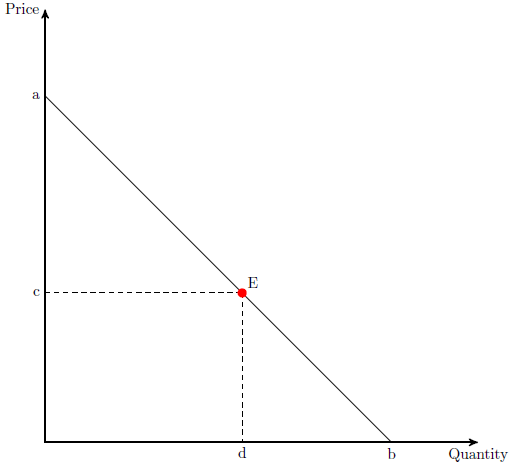
We can use the formula above, and note that the (absolute value of) PED at point E is:
\(
\begin{align*}
\epsilon_D &= \frac{ \Delta Q }{ \Delta P }\times \frac{P}{Q} \\
&= \frac{b-d}{c} \times \frac{c}{d} \\
&= \frac{b-d}{d}\\
\end{align*}
\)
Or, equivalently:
\(
\begin{align*}
\epsilon_D &= \frac{ \Delta Q }{ \Delta P }\times \frac{P}{Q} \\
&= \frac{d}{a-c} \times \frac{c}{d} \\
&= \frac{c}{a-c}\\
\end{align*}
\)
I am pretty sure it was Steve Salant who taught me this.
Updated Feb 2014: Steve Salant adds two more points. Firstly, that this trick also applies to nonlinear demand curves. Draw a tangent to the curve at the point of interest. Its slope will equal the slope of the curve at the point of tangency, and you can then follow the same procedure as above. Secondly, that the elasticity can be expressed in terms of either \(a\) and \(c\), or \(b\) and \(d\). I have altered the post to reflect this.