“Predictive capacity without explanatory capacity is worthless. Mere clairvoyance, irrespective of its sharpness, does not itself have scientific standing. Only predictive capacity that arises out of having coherent and communicable explanations has scientific standing. The power to predict is subsidiary to the power to explain. Explanation without prediction is sufficient, but prediction without explanation is of no consequence from a scientific standpoint.

— Harvey Leibenstein (1966), in “Beyond Economic Man”.

//

Ever have the problem of Stata regression output being a little too wide? Worry no more.

I use Ben Jann’s excellent esttab to export Stata regressions into LaTeX documents.

My only problem with esttab is that the tables can be too wide, i.e. wider than the width of the text in the PDF. So I made a few edits to esttab that automatically scale the tables to the text-width.

I have called this program estwide. You can download it here. As it is based on estout, Ben Jann should be considered a co-author. Click here to see an example of its effect. (If you wish to replicate the above example, you can download the associated do-file here and the TeX file here.)

To use estwide:
1. Make sure estout is installed. To do this, in Stata type ssc inst estout, replace
2. Save estwide.ado to the same folder that estout is now installed in. You can check the folder by typing which estout
3. Restart Stata.
4. Rather than exporting your tables using the esttab command, simply replace esttab with estwide, e.g. estwide using hello.tex, style(tex) replace
5. Make sure you have both the adjustbox and booktabs LaTeX packages installed.
6. Make sure you have called both of these packages up by including \usepackage{booktabs} and \usepackage{adjustbox} in the header of your LaTeX file.
7. Include your tables as normal. You can copy and paste the output into your TeX file, or have the tables update automatically when you make changes by using \input{myfilename}.

Update, September 2017: after some emails from people, I have two things to add. Firstly, estwide seems to work much better if you include a caption to the table.

Secondly, if you have a problem with the caption appearing on one page and the table itself on another, wrap the input in a LaTeX table. For example, this code works well for me:
\begin{table}[ht]
\input{myfilename}
\end{table}

//

“Consider now a participant in a social exchange economy. His problem has, of course, many elements in common with a [Robinson Crusoe] maximum problem. But it also contains some, very essential, elements of an entirely different nature. He too tries to obtain an optimum result. But in order to achieve this, he must enter into relations of exchange with others. If two or more persons exchange goods with each other, then the result for each one will depend in general not merely upon his own actions but on those of the others as well. Thus each participant attempts to maximize a function (his above-mentioned “results”) of which he does not control all variables. This is certainly no maximum problem, but a peculiar and disconcerting mixture of several conflicting maximum problems. Every participant is guided by another principle and neither determines all variables which affect his interest.

This kind of problem is nowhere dealt with in classical mathematics. We emphasize at the risk of being pedantic that this is no conditional maximum problem, no problem of the calculus of variations, of functional analysis, etc. It arises in full clarity, even in the most “elementary” situations, e.g. when all variables can assume only a finite number of values.

A particularly striking expression of the population misunderstanding about the pseudo-maximum problem is the famous statement according to which the purpose of the social effort is the “greatest possible good for the greatest possible number.” A guiding principle cannot be formulated by the requirement of maximizing two (or more) functions at once.

Such a principle, taken literally, is self-contradictory. (In general one function will have no maximum where the other function has one.) It is no better than saying, e.g., that a firm should obtain maximum prices at maximum turnover, or a maximum revenue at minimum outlay. If some order of importance of these principles or some weighted average is meant, this should be stated. However, in the situation of the participants in a social economy nothing of that sort is intended, but all maxima are desired at once–by various participants.

[…] Sometimes some of these interests run more or less parallel–then we are nearer to a simple maximum problem. But they can just as well be opposed. The general theory must cover all these possibilities, all intermediary stages, and all their combinations.”

— Von Neumann and Morgenstern (1944) — prior to Arrow-Debreu — on the “peculiar and disconcerting” properties of general equilibrium, on the motivation of game theory, and on political rhetoric.

//

“As the doctrine developed, the rule of equal marginal sacrifice soon won the day and with Pigou (1928, p. 60) became the correct solution. Viewed from the perspective of fairness, this was hardly persuasive. Why should only the marginal sacrifice be considered, rather than the entire loss as called for by equal-absolute, equal-proportional, or still other sacrifice rules? The answer, it appears, is that equal marginal sacrifice was chosen not so much as a matter of fairness but as an efficiency-based prescription for securing least total sacrifice. The move from Mill’s equal absolute or proportional sacrifice to Pigou’s enshrinement of equal marginal sacrifice thus involved a paradigm shift from equity to Pareto efficiency as the basic criterion. Equal marginal sacrifice, and with it least total sacrifice, fitted neatly into the economist’s utilitarian goal of welfare maximization. The case for distributing the burden of a given tax revenue so as to minimize aggregate loss was but a by-product of the general case for distributing income so as to maximize welfare. The entitlement base for distributive justice was thereby replaced by that of utilitarian welfare maximization.

[…] More basically, left open was the bottom-line question of why, as a matter of fairness or distributive justice, equal marginal sacrifice and hence least total sacrifice should be the accepted criterion. The case for least total sacrifice in tax-burden distribution, as Edgeworth and Pigou saw it, derives from the broader efficiency goal of securing a distribution of income which maximizes aggregate welfare. This takes us back to Bentham’s proposition that self-interested individuals, bent on maximizing their own welfare, will also wish to maximize aggregate welfare (Bentham 1789, p. 3), an heroic conclusion which hardly follows. Using superior force of bargaining from a stronger position, the self-interested and better-endowed individual would disagree, as Hobbes had put it in his “warre of everyone against every man” (1651, p. 188). To sustain acceptance, the target of maximum aggregate welfare had to be given an ethical underpinning. Based on the golden rule of valuing the welfare of others as one’s own, individuals should discard envy and agree to Pareto-optimal re-arrangements, that is, re-arrangements which produce a net gain for the group as a whole, even though the individual may lose. Given this more demanding premise of impartiality, least total sacrifice or welfare maximization becomes the preferred solution.

As formulated more recently, and in line with economists’ taste for maximizing behavior, impartiality has been interpreted as calling for choice under uncertainty.2 Individuals are called upon to choose among alternative patterns of distribution from behind a veil — that is, without knowing their own capacities and what their own position in any one pattern would be (Vickrey 1945; Harsanyi 1955; Rawls 1971). Assuming a fixed pie available for distribution and stipulating declining marginal utility or postulating risk aversion, people would then agree on an equal division of income; but, allowing for deadweight losses in response to taxation, some degree of inequality would be agreed on.3 Applying this reasoning to the narrower problem of just taxation, tax shares to be agreed upon from behind a veil would similarly fall short of maximum progression.

2 As I see it, the “veil” construct and the interpretation of distributive justice qua risk aversion, though congenial to the economist’s mode of thinking, is of questionable merit. If individuals have agreed on the principle of impartiality and thereby on the least-total-sacrifice rule, they should be willing to proceed directly to a corresponding income or tax-burden distribution. The veil construct becomes roundabout and redundant. Moreover, reliance on self-interested choice following disinterested acceptance of the veil seems inconsistent. This also poses the question of how acceptance of the impartiality premise (as distinct from the entitlement of earnings) can be reconciled with tax avoidance and the standing of the resulting deadweight loss (Musgrave 1992).

3 Viewed in this context, Rawls’s rule of maximin may be interpreted as involving extreme risk aversion.

— Richard A. Musgrave (1994), in his contribution to “Tax Progressivity and Income Inequality”, edited by Joel Slemrod.

//

“Economics is by its nature a softer and less exact science than, say, conventional physics. Now in a hard, exact science a practitioner does not really have to know much about methodology. Indeed, even if he is definitely a misguided methodologist, the subject itself has a self-cleaning property which renders harmless his aberrations. By contrast, a scholar in economics who is fundamentally confused concerning the relationship of definition, tautology, logical implication, empirical hypothesis, and factual refutation may spend a lifetime shadow-boxing with reality. In a sense, therefore, in order to earn his daily bread as a fruitful contributor to knowledge, the practitioner of an intermediately hard science like economics must come to terms with methodological problems. I stress the importance of intermediate hardness because when one descends lower still, say to certain areas of sociology that are almost completely without substantive content, it may not matter much one way or the other what truths or errors about scientific method are involved—for the reason that nothing matters.”

– Paul Samuelson, August 1964

//

I’ve been asked in the past for software recommendations. Almost all of these are standard.

My documents are almost always typeset in LaTeX. I use MiKTeX to compile the documents. MiKTeX is great, and free. I use beamer to generate presentations.

Before compiling documents, I use WinEdt to type them up. WinEdt works seamlessly with MiKTeX, and is a good all-round text editor. Its ability to select columns of text is often useful for coding. I think a student licence costs about $25.

I haven’t found a cloud storage system that’s better than Dropbox.

When dealing with data, I use Stata 90% of the time. In terms of getting Stata output into your document, the world owes a sincere debt of gratitude to Ben Jann for estout. Use estout to save your output as an external .tex file, and then \input{} it into your TeX code. It will automatically update the table the next time you compile.

Some things are easier done in R than in Stata. R is counter-intuitive for a lot of people. RStudio can make it easier. Both of these are free.

I use Mathematica to check any derivations for stray errors. It is from the same people who give us Wolfram Alpha. It can perform calculus/simplify symbolic algebra, so is a great tool for unwieldy models.

Rather than run loops in Stata, I often prefer to write loops in JavaScript that do the same thing. This is an idiosyncratic preference.

This blog runs on WordPress. It’s free. This website is hosted by Gandi, who I’ve had no problems with. I keep a track of who visits using the excellent (and free) StatCounter.com.

//

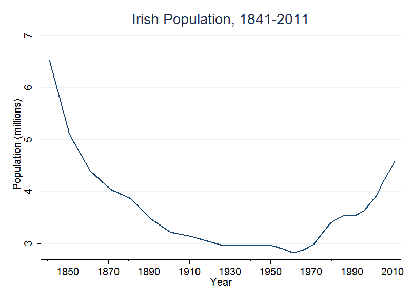
Using data from each Census since 1841, here’s a graph of Ireland’s population. For consistency this is the population of the Republic; what would become Northern Ireland is excluded. Often it is mentioned that the population declined by a quarter because of the Famine, but rarely is it noted that it fell by another quarter in the next generation as well.

It continued to fall for more than 100 years after 1850.

//

Are VATs regressive? No, not really.

People think that sales taxes (or Value Added Taxes) are regressive because rich people are able to save a higher proportion of their income than poor people. This is faulty reasoning.

Suppose we have two people (A and B), and a VAT rate of 10%. A earns $100,000 a year, and B earns $20,000 a year.

Here’s the argument people make:
“A earns $100,000 in a year, saves $30,000, and spends $70,000. With a VAT of 10%, and consumption of $70,000, $7,000 of his income that year goes to the government via VAT. That’s 7% of his income.

B earns $20,000 in a year and spends it all. That means that the government receives $2,000 a year from him in VAT. That’s 10% of his income.”

So it appears that the poor are paying more, as a fraction of their income, in VAT. That looks regressive.

But what this argument misses is that A’s savings of $30,000 do not simply disappear. He will spend it next year (or the year after, or the year after…) and will pay VAT on it. When he gets around to spending it he will pay $3,000 in VAT, which brings up his total contribution to $10,000, or exactly 10% of his income. Just like B.

You might wonder if this is still true if A earns interest on his savings. It turns out that it is: he will still pay 10% of his total income in VAT. Why? Assuming he eventually spends all of his money (or his kids do), then his consumption equals his income. Taxing the consumption at 10% means you are taxing the income at 10%.

There is one further implication of this regarding changes in VAT rates. If you think VATs are regressive, then you would probably like the VAT rate to be lowered. But doing so provides a tax-break to the people who are able to shift consumption to later periods, i.e. people who are rich enough to be able to save. Let’s go through an example. Again we have two people: A earns $100,000 a year and B earns $20,000 a year. But this time there are two years. In 2013 the VAT rate is 10%, and in 2014 it is lowered to 5%.

Mr A
In 2013: earns $100,000; puts $30,000 in a safe; spends $70,000. Pays $7,000 in VAT.
In 2014: earns $100,000; saves nothing; spends his income and the $30,000 he put in the safe, so spends $130,000. With the lower rate of 5%, he spends $6,500 in VAT.
Total VAT over two years = $13,500, or 6.75% of his total income.

Mr B
In 2013: earns $20,000; spends $20,000. Pays $2,000 in VAT.
In 2014: earns $20,000; spends $20,000. With the lower rate of 5%, he pays $1,000 in VAT.
Total VAT over two years = $3,000, or 7.5% of his overall income.

Lowering VATs can be regressive.
//

Undergrads are taught many formulae for the Price Elasticity of Demand. The most common one I have encountered is the particularly unwieldy “midpoint formula”:
\(\epsilon_D = \frac{ \frac{Q_2-Q_1}{(Q_1+Q_2)/2} }{\frac{P_2-P_1}{(P_1+P_2)/2}}\)

The elasticity at one point is a little more reasonable:
\(\epsilon_D = \frac{ \Delta Q }{ \Delta P }\times \frac{P}{Q}\)

There is an elegant simplification in the case of linear demand. With a demand curve like this:


We can use the formula above, and note that the (absolute value of) PED at point E is:
\(
\begin{align*}
\epsilon_D &= \frac{ \Delta Q }{ \Delta P }\times \frac{P}{Q} \\
&= \frac{b-d}{c} \times \frac{c}{d} \\
&= \frac{b-d}{d}\\
\end{align*}
\)
Or, equivalently:
\(
\begin{align*}
\epsilon_D &= \frac{ \Delta Q }{ \Delta P }\times \frac{P}{Q} \\
&= \frac{d}{a-c} \times \frac{c}{d} \\
&= \frac{c}{a-c}\\
\end{align*}
\)

I am pretty sure it was Steve Salant who taught me this.

Updated Feb 2014: Steve Salant adds two more points. Firstly, that this trick also applies to nonlinear demand curves. Draw a tangent to the curve at the point of interest. Its slope will equal the slope of the curve at the point of tangency, and you can then follow the same procedure as above. Secondly, that the elasticity can be expressed in terms of either \(a\) and \(c\), or \(b\) and \(d\). I have altered the post to reflect this.

//
Scroll to Top